这篇文章主要记述了MATLAB。
1、首先把照片中每一个偏振角度里的值抠出来赋给im ,然后通过一个遮罩获取通过的像素点放到I 的列向量里。
1 | for i=1:nimages |
2、进入线性方法中,生成一个(偏振角度)行 3 列的矩阵A【第一列是单位1,第二列是偏振角度的余弦,第三列是偏振角度的正弦】
A = [ones(nimages,1) cos(2.*angles') sin(2.*angles')];
3、一般情况下,x=a\b是方程ax =b的解,而x=b/a是方程xa=b的解
1 | x = A\(I');% A * x = (I') I' = 36行*74331列 A 36行3列 |
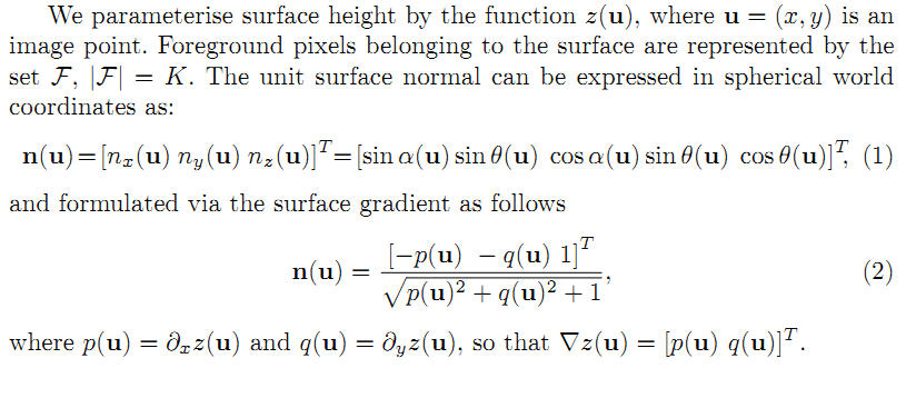
Linear depth estimation from an uncalibrated,monocular polarisation image
To do so, we show how to express polarisation constraints as equations that are linear in the unknown depth.The ambiguity in the surface normal azimuth angle is resolved globally when the optimal surface height is reconstructed.
Our method is applicable to objects with uniform albedo exhibiting diffuse and specular reflectance.
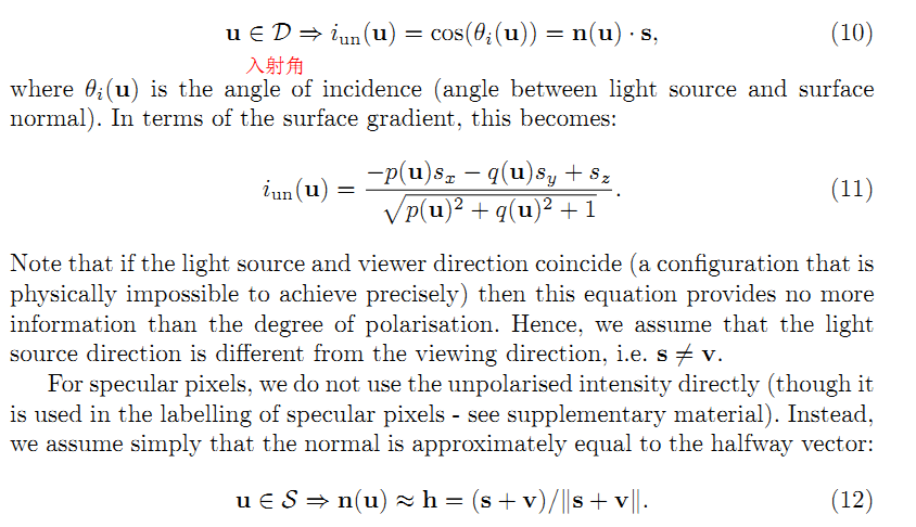
我们的方法适用于具有均匀漫反射率的物体,这些物体具有漫反射和镜面反射。
We extend it to an uncalibrated scenario by demonstrating that the illumination (point source or first/second order spherical harmonics) can be estimated from the polarisation image, up to a binary convex/concave ambiguity. We believe that our method is the first monocular, passive shape-from-x technique that enables well-posed depth estimation with only a single, uncalibrated illumination condition. We present results on glossy objects, including in uncontrolled, outdoor illumination.
通过证明可以从偏振图像估计照度(点源或一阶/二阶球面谐波),直至二元凸/凹歧义性,我们将其扩展到未经校准的情况。
我们相信,我们的方法是第一种单眼,被动x形技术,该技术仅用一个未经校准的照明条件即可进行精确的深度估计。
我们介绍了有光泽物体的结果,包括不受控制的室外照明。
- In contrast to prior work, we compute SfP in the depth, as opposed to the
surface normal, domain. Instead of disambiguating the polarisation normals,
we defer resolution of the ambiguity until surface height is computed. To do
so, we express the azimuthal ambiguity as a collinearity condition that is
satisfied by either interpretation of the polarisation measurements. - We express polarisation and shading constraints as linear equations in the
unknown depth enabling e!cient and globally optimal depth estimation. - We use a novel hybrid di↵use/specular polarisation and shading model, al-
lowing us to handle glossy surfaces. - We show that illumination can be determined from the ambiguous normals
and unpolarised intensity up to a binary ambiguity (a particular generalised
Bas-relief [4] transformation: the convex/concave ambiguity). This means
that our method can be applied in an uncalibrated scenario and we consider
both point source and 1st/2nd order spherical harmonic (SH) illumination.
1.不同于前面那些人的工作,本文采用深度进行计算而不是采用表面法向量进行计算。除了消除极化法线的歧义外,我们将方位角的去歧义性工作推迟到计算出表面高度为止。
2.我们将偏振和阴影约束表示为未知深度中的线性方程,从而能够进行有效且全局最佳的深度估计
3.我们使用了一种新颖的混合漫反射/镜面偏振和阴影模型,使我们能够处理光滑的表面。
4.我们表明,可以从模态不明确的法线和非极化强度直至二元模糊度(特定的广义Bas-relief [4]变换:凸/凹模糊度)确定照明。
这意味着我们的方法可以应用于未经校准的场景,并且我们同时考虑了点光源和一阶/二阶球谐(SH)照明。
SFP 可以分成单纯使用偏振图片的和与其他器件混合使用的(Kinect),还可以分成只考虑漫反射的,只考虑镜面反射的,两者混合考虑的,还可以分成从表面法线域考虑的和从表面深度域进行考虑的。
光照约束
这个非极化强度通过适当的反射模型在表面法线方向上提供了附加约束。我们假设,对于带有漫反射标签的像素,根据朗伯模型对光进行反射。我们还假设反照率是均匀的,并将其分解为光源向量s。
因此,非极化强度与表面法线的关系如下:
首先,我们注意到相位角约束可以写为共线性条件。
通过相角测量所隐含的两个可能的方位角中的任何一个都可以满足这种条件。
以这种方式编写它是有利的,因为它意味着我们不必明确消除表面法线的歧义。
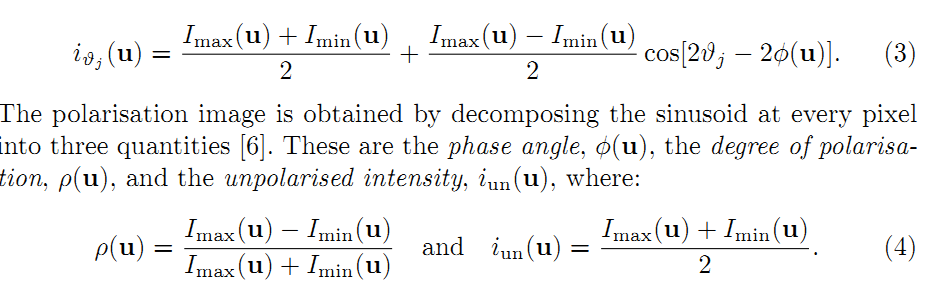
原数据集与已知点光源
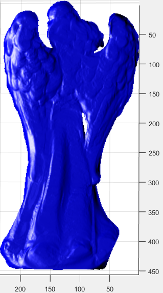
原数据集与未知点光源
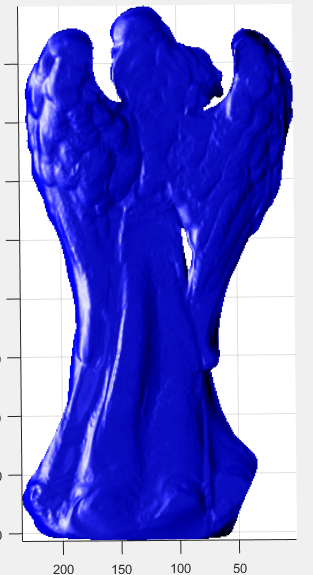
忽略镜面反光与遮罩与未知光源


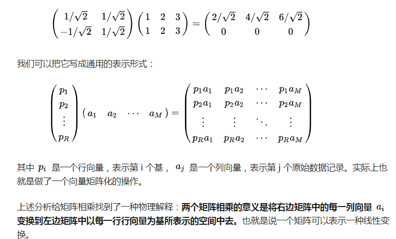
两个矩阵相乘的意义是将右边矩阵中的每一列向量 ai 变换到左边矩阵中以每一行行向量为基所表示的空间中去。
在一维空间中我们可以用方差来表示数据的分散程度。而对于高维数据,我们用协方差进行约束,协方差可以表示两个变量的相关性。为了让两个变量尽可能表示更多的原始信息,我们希望它们之间不存在线性相关性,因为相关性意味着两个变量不是完全独立,必然存在重复表示的信息。
协方差公式为:
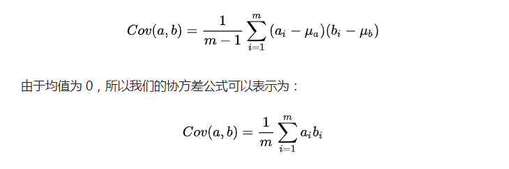
当协方差为 0 时,表示两个变量完全独立。为了让协方差为 0,我们选择第二个基时只能在与第一个基正交的方向上进行选择,因此最终选择的两个方向一定是正交的。
至此,我们得到了降维问题的优化目标:将一组 N 维向量降为 K 维,其目标是选择 K 个单位正交基,使得原始数据变换到这组基上后,各变量两两间协方差为 0,而变量方差则尽可能大(在正交的约束下,取最大的 K 个方差)。
总结一下 PCA 的算法步骤:
设有 m 条 n 维数据。
- 将原始数据按列组成 n 行 m 列矩阵 X;
- 将 X 的每一行进行零均值化,即减去这一行的均值;
- 求出协方差矩阵
;
- 求出协方差矩阵的特征值及对应的特征向量;
- 将特征向量按对应特征值大小从上到下按行排列成矩阵,取前 k 行组成矩阵 P;
即为降维到 k 维后的数据。